Continuing the Pytorch series, in this post we’ll learn about how non-linearities help solve complex problems in the context of neural networks

In the last blog posts of the PyTorch Introduction series, we spoke about introduction to tensor objects and building a simple linear model using PyTorch. The first two blog posts of the series were the start of a larger objective where we understand deep learning at a deeper level (pun intended). To do that, we are using one of the most famous libraries in the machine learning world, PyTorch.

When building our simple linear model, we’ve understood that PyTorch is able to solve simple regression problems — but it wouldn’t be a deep learning library if these would be the only problems that it could solve, right? In this blog post, we are going to go a bit deeper into the complexities of Neural Networks and learn a bit about how to implement a neural network that deals with non-linear patterns and solve complex problems by introducing the concept of activation functions.

This blog post (and series) is loosely based on the structure of https://www.learnpytorch.io/, an excellent resource to learn PyTorch that I recommend you to check out!

In a nutshell, in this blog post, we will:

• Understand how activation functions in PyTorch work.
• Explore how we can solve a non-linear problem using Neural Networks.

Let’s start!

Setting up our Data

In this blog post, we’ll use the Heart Failure prediction dataset available at Kaggle. The dataset contains data from 299 patients with heart failure and specifies different variables about their health status. The goal is to predict if the patients died (column named DEATH_EVENT) and understand if there’s any signal in the patient’s Age, Anaemia level, ejection fraction or other health data that can predict the death outcome.

Let’s start by loading our data using pandas :

import pandas as pd
heart_failure_data = pd.read_csv('heart_failure_clinical_records_dataset.csv')

Let’s see the head of our DataFrame:

heart_failure_data.head(10)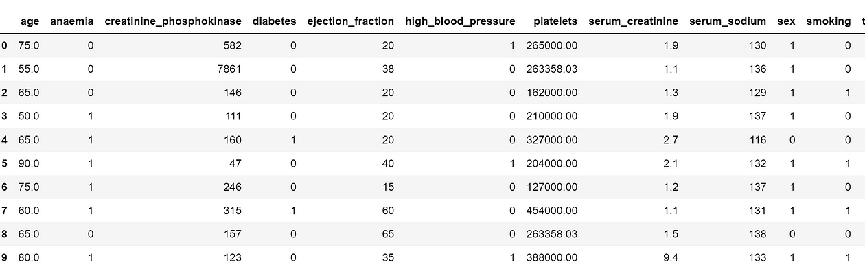

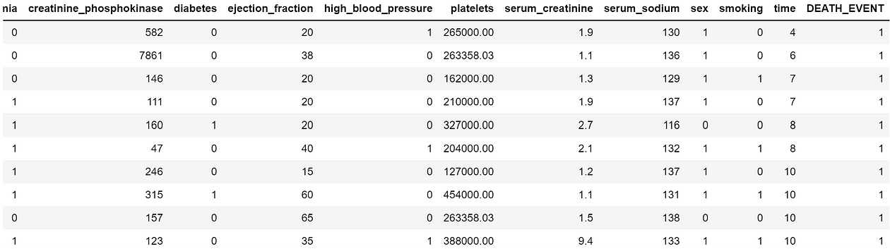
Our goal is to predict the DEATH_EVENT binary column, available at the end of the DataFrame:

First, let’s standardize our data using StandardScaler — although not as important as in distance algorithms, standardizing the data will be extremely helpful to improve the gradient descent algorithm we’ll use during the training process. We’ll want to scale all but the last column (the target):

from sklearn.preprocessing import StandardScaler

scaler = StandardScaler()
heart_failure_data_std = scaler.fit_transform(heart_failure_data.iloc[:,:-1])

Now, we can perform a simple train-test split. We’ll use sklearn to do that and leave 20% of our dataset for testing purposes:

X_train, X_test, y_train, y_test = train_test_split(
    heart_failure_data_std, heart_failure_data.DEATH_EVENT, test_size = 0.2, random_state=10
)

We also need to transform our data into torch.tensor :

X_train = torch.from_numpy(X_train).type(torch.float)
X_test = torch.from_numpy(X_test).type(torch.float)
y_train = torch.from_numpy(y_train.values).type(torch.float)
y_test = torch.from_numpy(y_test.values).type(torch.float)

Having our data ready, time to fit our Neural Network!

Training a Vanilla Linear Neural Network

With our data in-place, it’s time to train our first Neural Network. We’ll use a similar architecture to what we’ve done in the last blog post of the series, using a Linear version of our Neural Network with the ability to handle linear patterns:

from torch import nn

class LinearModel(nn.Module):
    def __init__(self):
        super().__init__()
        self.layer_1 = nn.Linear(in_features=12, out_features=5)
        self.layer_2 = nn.Linear(in_features=5, out_features=1)
    
    def forward(self, x):
        return self.layer_2(self.layer_1(x))

This neural network uses the nn.Linearmodule from pytorch to create a Neural Network with 1 deep layer (one input layer, a deep layer and an output layers).

Although we can create our own class inheriting from nn.Module , we can also use (more elegantly) the nn.Sequential constructor to do the same:

model_0 = nn.Sequential(
 nn.Linear(in_features=12, out_features=5),
 nn.Linear(in_features=5, out_features=1)
)

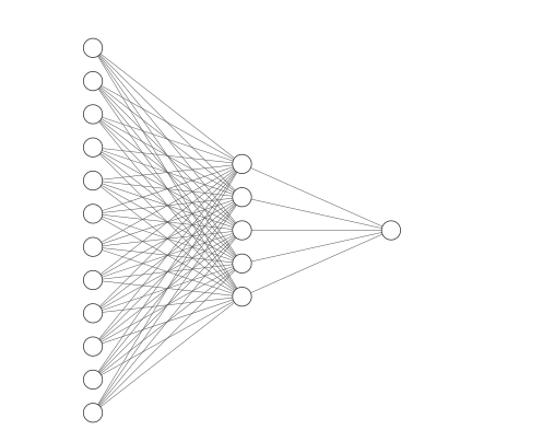
Cool! So our Neural Network contains a single inner layer with 5 neurons (this can be seen by the out_features=5 on the first layer).

This inner layer receives the same number of connections from each input neuron. The 12 in in_features in the first layer reflects the number of features and the 1 in out_features of the second layer reflects the output (a single value raging from 0 to 1).

To train our Neural Network, we’ll define a loss function and an optimizer. We’ll define BCEWithLogitsLoss (PyTorch 2.1 documentation) as this loss function (torch implementation of Binary Cross-Entropy, appropriate for classification problems) and Stochastic Gradient Descent as the optimizer (using torch.optim.SGD ).

# Binary Cross entropy
loss_fn = nn.BCEWithLogitsLoss()

# Stochastic Gradient Descent for Optimizer
optimizer = torch.optim.SGD(params=model_0.parameters(), 
 lr=0.01)

Finally, as I’ll also want to calculate the accuracy for every epoch of training process, we’ll design a function to calculate that:

def compute_accuracy(y_true, y_pred):
    tp_tn = torch.eq(y_true, y_pred).sum().item()
    acc = (tp_tn / len(y_pred)) * 100 
    return acc

Time to train our model! Let’s train our model for 1000 epochs and see how a simple linear network is able to deal with this data:

torch.manual_seed(42)

epochs = 1000

train_acc_ev = []
test_acc_ev = []

# Build training and evaluation loop
for epoch in range(epochs):

    model_0.train()

    y_logits = model_0(X_train).squeeze()
    
    loss = loss_fn(y_logits,
                   y_train) 
    # Calculating accuracy using predicted logists
    acc = compute_accuracy(y_true=y_train, 
                      y_pred=torch.round(torch.sigmoid(y_logits))) 
    
    train_acc_ev.append(acc)

    # Training steps
    optimizer.zero_grad()
    loss.backward()
    optimizer.step()
    model_0.eval()
    
    # Inference mode for prediction on the test data
    with torch.inference_mode():
        
        
        test_logits = model_0(X_test).squeeze() 
        test_loss = loss_fn(test_logits,
                            y_test)
        test_acc = compute_accuracy(y_true=y_test,
                               y_pred=torch.round(torch.sigmoid(test_logits)))
        test_acc_ev.append(test_acc)
    
    # Print out accuracy and loss every 100 epochs
    if epoch % 100 == 0:
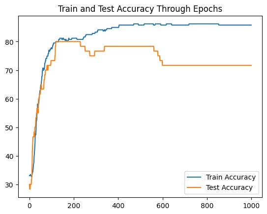
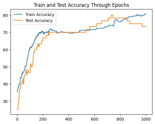
        print(f"Epoch: {epoch}, Loss: {loss:.5f}, Accuracy: {acc:.2f}% | Test loss: {test_loss:.5f}, Test acc: {test_acc:.2f}%")

Unfortunately the neural network we’ve just built is not good enough to solve this problem. Let’s see the evolution of training and test accuracy:

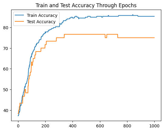
(I’m plotting accuracy instead of loss as it is easier to interpret in this problem)

Interestingly, our Neural Network isn’t able improve much of the test set accuracy.

With the knowledge have from previous blog posts, we can try to add more layers and neurons to our neural network. Let’s try to do both and see the outcome:

deeper_model = nn.Sequential(
 nn.Linear(in_features=12, out_features=20),
 nn.Linear(in_features=20, out_features=20),
 nn.Linear(in_features=20, out_features=1)
)

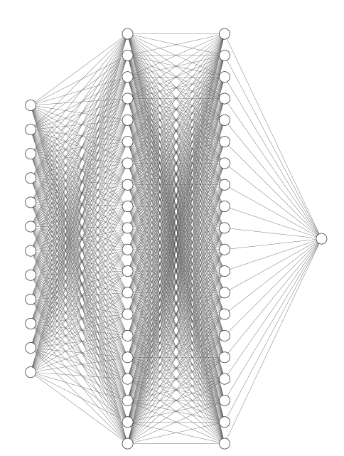
Although our deeper model is a bit more complex with an extra layer and more neurons, that doesn’t translate into more performance in the network:

Even though our model is more complex, that doesn’t really bring more accuracy to our classification problem.

To be able to achieve more performance, we need to unlock a new feature of Neural Networks — activation functions!

Enter NonLinearities!

If making our model wider and larger didn’t bring much improvement, there must be something else that we can do with Neural Networks that will be able to improve its performance, right?

That’s where activation functions can be used! In our example, we’ll return to our simpler model, but this time with a twist:

model_non_linear = nn.Sequential(
 nn.Linear(in_features=12, out_features=5),
 nn.ReLU(),
 nn.Linear(in_features=5, out_features=1)
)

What’s the difference between this model and the first one? The difference is that we added a new block to our neural network — nn.ReLU . The rectified linear unit is an activation function that will change the calculation in each of the weights of the Neural Network:

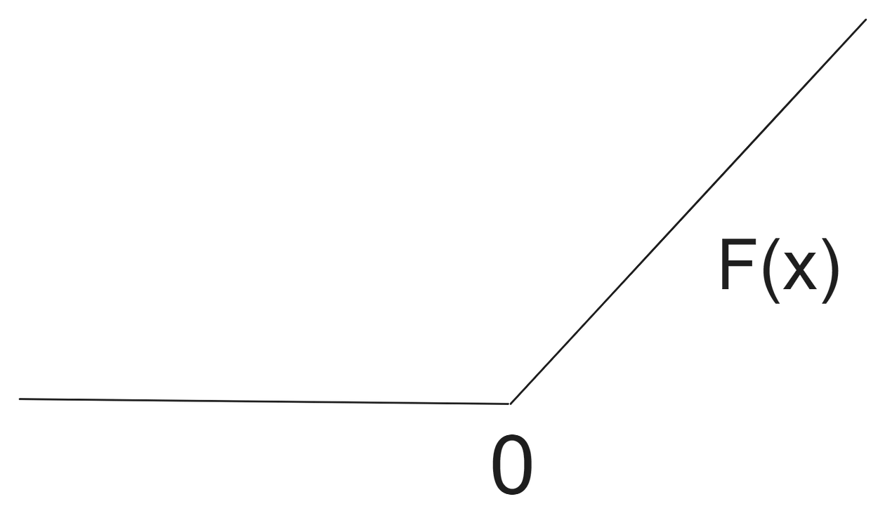
Every value that goes through our weights in the Neural Network will be computed against this function. If the value of the feature times the weight is negative, the value is set to 0, otherwise the calculated value is assumed. Just this small change adds a lot of power to a Neural Network architecture — in torch we have different activation functions we can use such as nn.ReLU , nn.Tanh or nn.ELU . For an overview of all activation functions, check this link.

Our neural network architecture contains a small twist, at the moment:

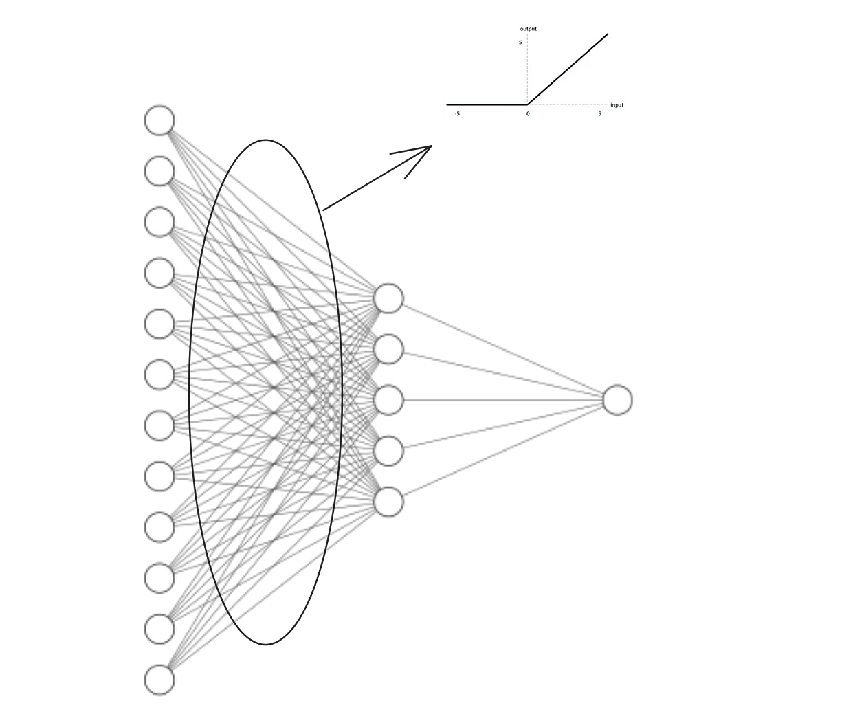
With this small twist in the Neural Network, every value coming from the first layer (represented by nn.Linear(in_features=12, out_features=5) ) will have to go through the “ReLU” test.

Let’s see the impact of fitting this architecture on our data:

Cool! Although we see some of the performance degrading after 800 epochs, this model doesn’t exhibit overfitting as the previous ones. Keep in mind that our dataset is very small, so there’s a chance that our results are better just by randomness. Nevertheless, adding activation functions to your torch models definitely has a huge impact in terms of performance, training and generalization, particularly when you have a lot of data to train on.

Now that you know the power of non-linear activation functions, it’s also relevant to know:

• You can add activation functions to every layer of the Neural Network.
• Different activation functions have different effects on your performance and training process.
• torch elegantly gives you the ability to add activation functions in-between layers by leveraging the nn module.

Conclusion

Thank you for taking the time to read this post! In this blog post, we’ve checked how to incorporate activation functions inside torch Neural Network paradigm. Another important concept that we’ve understood is that larger and wider networks are not a synonym of better performance.

Activation functions help us deal with problems that are solved with more complex architectures (again, more complex is different than larger/wider). They help with generalization power and help us converge our solution faster, being one of the major features of neural network models.

And because of their widespread use on a variety of neural models, torch has got our back with its cool implementation of different functions inside the nn.Sequential modules!

Hope you’ve enjoyed and see you on the next PyTorch post! You can check the first PyTorch blog posts here and here. I also recommend that you visit PyTorch Zero to Mastery Course, an amazing free resource that inspired the methodology behind this post. Also, feel free to check our PyTorch Fundamentals repo.

[The dataset used in this blog post is under licence Creative Commons https://bmcmedinformdecismak.biomedcentral.com/articles/10.1186/s12911-020-1023-5#Sec2]