

In this post, we’ll learn how to train a computer vision model using a convolutional Neural Network in PyTorch
PyTorch is currently one of the hottest libraries in the Deep Learning field. Used by thousand of developers around the world, the library gained prominence since the release of ChatGPT and the introduction of deep learning into mainstream news headlines.
With its capabilities of efficiently training deep learning models (with GPU-ready features), it has become a machine learning engineer and data scientist’s best friend when it comes to train complex neural network algorithms.
So far, in this PyTorch series, we’ve covered several fundamentals that gave us the foundations to work with this library from scratch. For example:
- We’ve learned the basics about tensors;
- We understood how to create our first linear model (regression) using PyTorch.
- We’ve learned how to work with non-linear activation functions and how to solve non-linear problems.
- We’ve seen how to use custom data in the context of the library.
In this blog post, we are finally going to bring out the big guns and train our first computer vision algorithm. Alongside, we’ll also get to know convolutional neural networks (CNNs), a famous set of architectures tailored for training computer vision models. Although we’ll use a simple dataset here (making it accessible for anyone to run this code on their computer), the principles we’ll see can be applied to other image classification algorithms.
Let’s start!
Loading and Preparing the Data
As a way for everyone to be able to run this pipeline without the need for a GPU, we’ll keep it simple and use the ever-present MNIST dataset.
This dataset consists of handwritten digits and is available in torchvision by running the following code:
import torchvision
from torchvision.transforms import transforms

transform = transforms.Compose([
    transforms.ToTensor(),
    transforms.Normalize((0.5,), (0.5,))
])

# Load training and test datasets
train_dataset = torchvision.datasets.MNIST(root='./data', train=True, download=True, transform=transform)
test_dataset = torchvision.datasets.MNIST(root='./data', train=False, download=True, transform=transform)
Note: I’ll add the imports we need during the code for visualization purposes, but the recommendation is that you always put them on top of your code
torchvision.datasets also has another cool feature: we can immediately add a transform that will be applied directly to images. In our case, our transform pipeline will:
- Transform our data to tensor;
- Normalize the data;
Although not very important for this grayscale dataset (as it only contains one channel of color) normalization will definitely help the gradient descent process and prevent exploding or vanishing gradients during the training of our models.
With our datasets in memory, it’s time to see what our tensors contain! Let’s take a look at the first one:
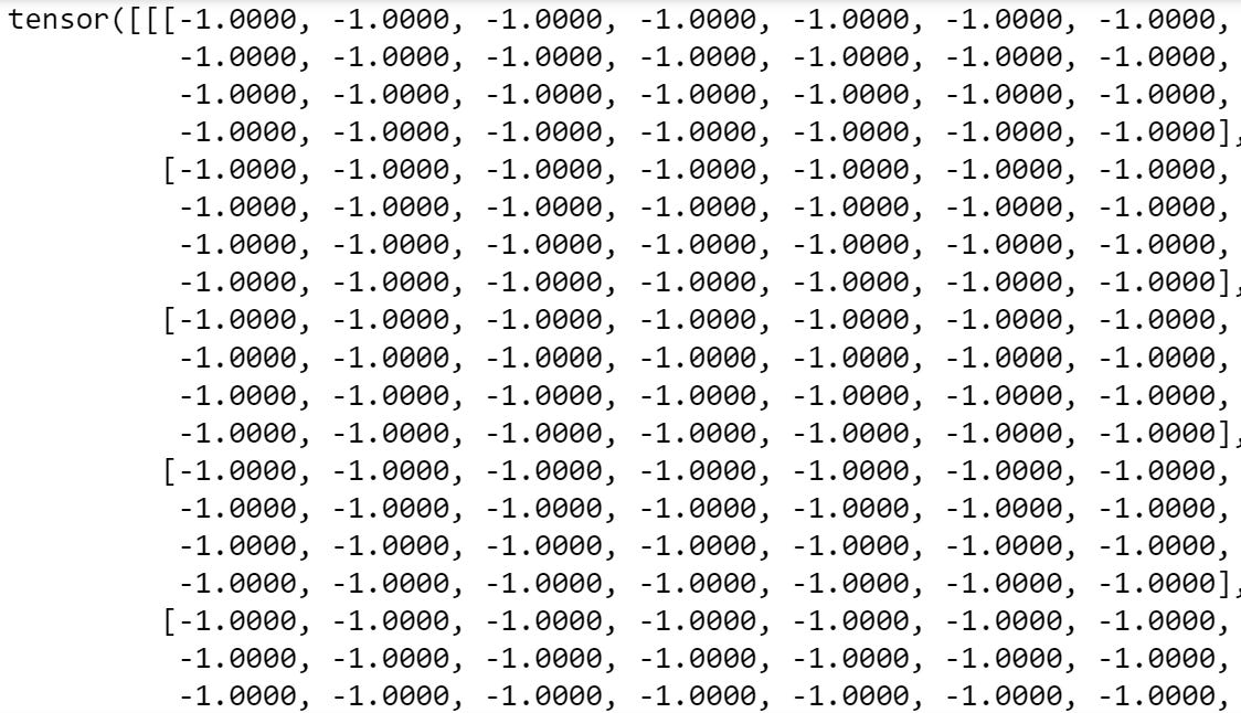
Errr.. ok, hard to visualize! let’s see the shape of the tensor:
We have a 28 x 28 tensor of 1 channel. Maybe it’s better to visualize our tensor in image format! Let’s do that:
import matplotlib.pyplot as plt
import numpy as np

image, label = train_dataset[0]
image = np.transpose(image, (1, 2, 0))
plt.figure(figsize=(4, 4))
plt.imshow(image)
plt.title(label);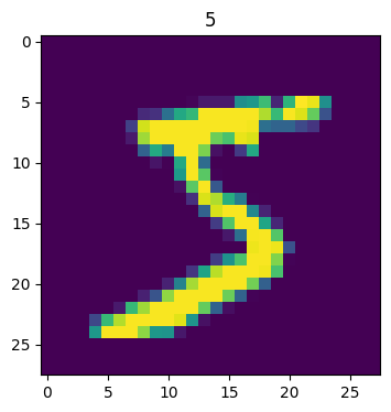
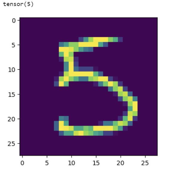
We have the number 5 in the first row! Let’s see another tensor in the dataset:
image, label = train_dataset[120]
image = np.transpose(image, (1, 2, 0))
plt.figure(figsize=(4, 4))
plt.imshow(image)
plt.title(label);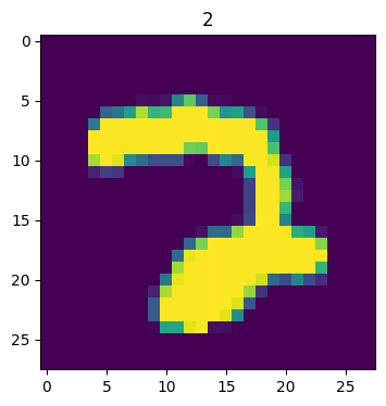
Number 2!
Now, our goal is to classify these numbers with the correct digit. Basically, our algorithm will have to check, based on these tensors, how to classify the number on the image.
As usual, in pytorch, we need to use batches to feed the data to our neural network — if we need it, torch has it!
import torch

train_loader = torch.utils.data.DataLoader(train_dataset, batch_size=30, shuffle=True)
test_loader = torch.utils.data.DataLoader(test_dataset, batch_size=30)
We’re using 30 examples on each batch. This will help us train our neural network, next.
With our data in-place, let’s create our model!
Creating a Standard Neural Network Model
Before training our model, let’s see the classes that our model will need to classify:
class_names = train_dataset.classes
class_names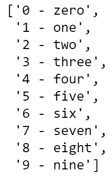
So our first algorithm will be super simple — a single hidden layer with ReLU activation. If this sentence sounds odd to you, consider visiting the other blog posts of this series, which are linked in the introduction!
class MNIST_NN(nn.Module):
    def __init__(self, input_shape: int,
                 hidden_units: int,
                 output_shape: int):
        super().__init__()

        # Create a hidden layer with non-linearities
        self.layer_stack = nn.Sequential(
            nn.Flatten(),
            nn.Linear(in_features=input_shape, out_features=hidden_units),
            nn.ReLU(),
            nn.Linear(in_features=hidden_units, out_features=output_shape),
            nn.ReLU()
        )

    def forward(self, x: torch.Tensor):
        return self.layer_stack(x)
We’ll use 150 units in our hidden layer:
model_non_linear = MNIST_NN(input_shape=28*28,
 hidden_units=150,
 output_shape=len(class_names))
As a loss function, we’ll use CrossEntropy (suitable for classification problems) and we will use stochastic gradient descent optimizer (with 0.01 learning rate):
loss_function = nn.CrossEntropyLoss()
optimizer = torch.optim.SGD(params=model_1.parameters(),
 lr=0.01)
Time to define our train and test steps next:
def train_step(model: torch.nn.Module,
               data_loader: torch.utils.data.DataLoader,
               loss_fn: torch.nn.Module,
               optimizer: torch.optim.Optimizer,
               accuracy_fn):

    # Zero loss and acc
    train_loss, train_acc = 0, 0

    model.train()

    for batch, (X, y) in enumerate(data_loader):

        y_pred = model(X)
        loss = loss_fn(y_pred, y)
        train_loss += loss.item()
        train_acc += accuracy_fn(y_true=y,
                                 y_pred=y_pred.argmax(dim=1))

        optimizer.zero_grad()
        loss.backward()
        optimizer.step()

    train_loss /= len(data_loader)
    train_acc /= len(data_loader)
    print(f"Train loss: {train_loss:.2f} | Train accuracy: {train_acc:.2f}%")

    return train_loss

def test_step(data_loader: torch.utils.data.DataLoader,
              model: torch.nn.Module,
              loss_fn: torch.nn.Module,
              accuracy_fn):
    test_loss, test_acc = 0, 0
    model.eval()

    with torch.no_grad():
        for X, y in data_loader:
            test_pred = model(X)
            test_loss += loss_fn(test_pred, y).item()
            test_acc += accuracy_fn(y_true=y,
                                    y_pred=test_pred.argmax(dim=1))

        test_loss /= len(data_loader)
        test_acc /= len(data_loader)
        print(f"Test loss: {test_loss:.5f} | Test accuracy: {test_acc:.2f}%\n")

        return test_loss
These steps have been approached in our Training a Linear Model blog post. Feel free to revisit it if you are finding this difficult to grasp!
In a nutshell, we are creating the training and step processes that will help our neural network perform back-propagation.
Alright, everything is in its place. Time to train our feed-forward NN model:
loss_hist = {}

loss_hist['train'] = {}
loss_hist['test'] = {}

epochs = 10
for epoch in tqdm(range(epochs)):
    print(f"Epoch: {epoch}\n---------")
    train_loss = train_step(data_loader=train_loader,
        model=model_non_linear,
        loss_fn=loss_function,
        optimizer=optimizer,
        accuracy_fn=accuracy_fn
    )

    loss_hist['train'][epoch] = train_loss

    test_loss = test_step(data_loader=test_loader,
        model=model_non_linear,
        loss_fn=loss_function,
        accuracy_fn=accuracy_fn
    )

    loss_hist['test'][epoch] = test_loss
We’ll train it for 10 epochs. Remember that a training epoch is a complete pass on the data, so our neural network will see each example 10 times. After a while (depending on your system’s resources), the neural network should finish the training process:
We could probably continue to train our neural network for a while as it seems that the loss still had some points room for further improvement past 10 epochs.
In terms of accuracy, let’s see the status of the accuracy and loss in the last epoch:
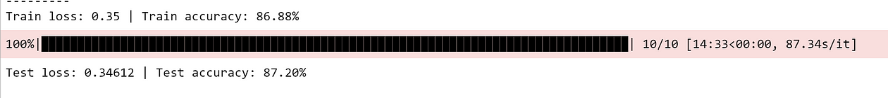
Cool, around 87% accuracy and our model isn’t showing signs of overfit!
Finally, let’s pass some handwritten images through the algorithm and see how it’s performing in the classification of digits. For that, we’ll use a custom show_predict_digit function:
def show_predict_digit(model, dataset, index):
    image_tensor = dataset.data[index].unsqueeze(0).unsqueeze(0).to(torch.float32)
    plt.figure(figsize=(4, 4))
    plt.imshow(image_tensor.squeeze(0).squeeze(0))

    with torch.no_grad():
        output = model(image_tensor)

    return torch.argmax(output)
Starting with the digit on index 0 in our test set:
show_predict_digit(model_non_linear,
 test_dataset,
 0)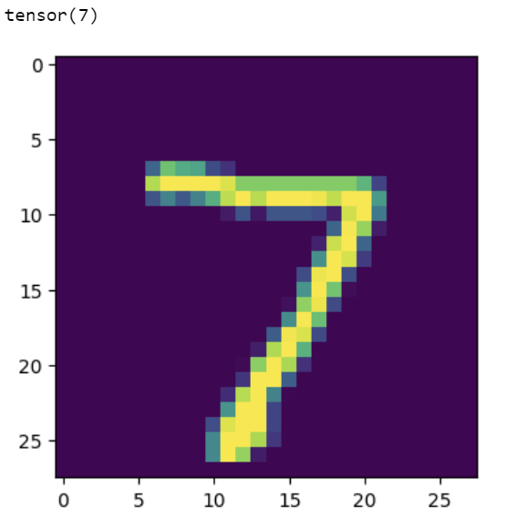
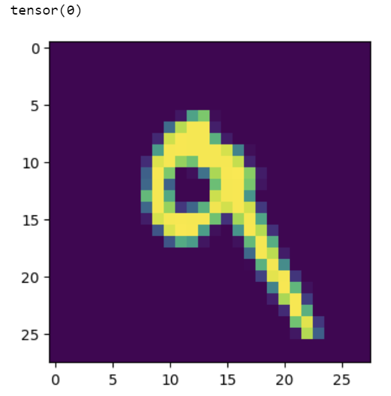
Right above the image, do you see “tensor(7)”? This is the output from our neural network. In a perfect world, this would match the digit we are seeing on the screen, everytime.
In this case, we got this digit correctly! Our neural network is predicting the digit 7. Let’s see another example:
Too bad! :-( As our image highlights the circle on the digit “9”, our neural network is incorrectly classifying the digit as “0”. There’s certainly still some room for improvement in the algorithm!
It’s expected that feed-forward neural networks exhibit this behavior, particularly in problems that suffer from large dimensionality (such as image classification that rely on pixel-by-pixel features).
In the next part of this blog post, we’ll try to solve this issue by fitting our first convolutional neural network, a specific type of neural network that is tailored to deal with computer vision problems.
Training a Convolutional Neural Network
Let’s now build a new neural network model using pytorch— in this case, we’re going to use a convolutional neural network (CNN).
These types of neural network architectures are tailored for vision algorithms and to work with high dimensionality data. When it comes to image data, they focus on specific features within the image with its architecture being loosely inspired by the human eye.
Some of the most famous operations of a CNN are pooling, sampling and flatten operations — they help our algorithm converge faster and with less error. Explaining convolutional neural networks is outside of the scope of this post, but you can check this awesome blog post on TDS and this great visualizer on how data passes through the layers of a CNN.
class SimpleCNN(nn.Module):
    def __init__(self):
        super(SimpleCNN, self).__init__()
        self.conv1 = nn.Conv2d(in_channels=1, out_channels=32,
                               kernel_size=3, padding=1)
        self.conv2 = nn.Conv2d(32, 64, kernel_size=3, padding=1)
        self.pool = nn.MaxPool2d(kernel_size=2, stride=2)
        self.fc1 = nn.Linear(64 * 7 * 7, 128)
        self.fc2 = nn.Linear(128, 10)
        self.dropout = nn.Dropout(0.5)
        self.batch_norm1 = nn.BatchNorm2d(32)
        self.batch_norm2 = nn.BatchNorm2d(64)

    def forward(self, x):
        x = self.pool(F.relu(self.batch_norm1(self.conv1(x))))
        x = self.pool(F.relu(self.batch_norm2(self.conv2(x))))
        x = torch.flatten(x, 1)
        x = F.relu(self.fc1(x))
        x = self.dropout(x)
        x = self.fc2(x)
        return x
In our convolutional neural network, we have the following architecture:
- A normalized convolutional layer with a 3 by 3 kernel and 32 output channels.
- A pooling operation with RELU activation, processed in
self.pool(F.relu(self.batch_norm1(self.conv1(x)))) - A second normalized convolutional layer with a 3 by 3 kernel.
- A pooling operation with RELU activation, processed in
self.pool(F.relu(self.batch_norm2(self.conv2(x)))) - A flattening layer —
torch.flatten(x,1) - Finally, two fully connected layers with a dropout in-between to prevent overfit.
Training a CNN in pytorch is similar to training a typical feed-forward neural network:
net = SimpleCNN()

optimizer = torch.optim.SGD(params=net.parameters(),
                            lr=0.05)
In this example, we’ll be using stochastic gradient descent with 0.05learning rate. We can rely on code we previously defined to train the network:
loss_hist_cnn = {}

loss_hist_cnn['train'] = {}
loss_hist_cnn['test'] = {}

epochs = 10
for epoch in tqdm(range(epochs)):
    print(f"Epoch: {epoch}\n---------")
    loss_cnn = train_step(data_loader=train_loader,
        model=net,
        loss_fn=loss_function,
        optimizer=optimizer,
        accuracy_fn=accuracy_fn
    )

    loss_hist_cnn['train'][epoch] = loss_cnn

    loss_cnn_test = test_step(data_loader=test_loader,
        model=net,
        loss_fn=loss_function,
        accuracy_fn=accuracy_fn
    )

    loss_hist_cnn['test'][epoch] = loss_cnn_test
After our 10th epoch, these are the results of our accuracy and loss:

Cool! It seemed we improved our model’s accuracy by a lot, by more than 10 percentage points. This is clearly outperforming the simple non-linear architecture.
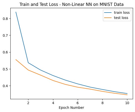
Let’s confirm that by plotting the train and test loss curves:
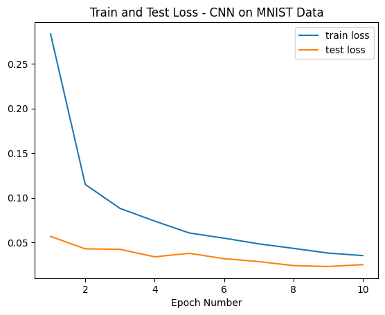
We have the confirmation that loss is lower than the first experiment. But, we’ll not celebrate yet! It’s time for the litmus test: let’s see how our model is classifying the “9" digit that our first classifier was predicting incorrectly:
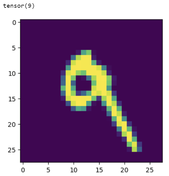
So cool! We’re now able to predict this digit correctly using a CNN. To wrap things up and out of curiosity, let’s see another random example:
show_predict_digit_cnn(net,
                  test_dataset,
                  15)
Another example correct! Can you check more digits and see if you can find the rare cases where our CNN is falling?
And that’s a wrap for this post! Thank you for reading until the end and I hope that these examples helped you understand how to train a convolutional neural network using pytorch . It was also our first time dealing with these types of layers within the framework and it’s really cool to see how torch is built similar to lego bricks! As soon as you understand how the layers work, mixing and matching them will give you extraordinary abilities when it comes to building deep learning models.
In summary, here’s what we’ve done in this blog post:
- Trained our first computer vision model
- Fitted a typical feed-forward neural network on the MNIST dataset
- Fitted a CNN on the MNIST dataset
- Touched lightly upon the concept of CNNs and got to know conv, flatten, and pool layers.
Hope you’ve enjoyed this and see you on the next PyTorch post!
You can check the first PyTorch blog posts from this series here and here. I also recommend that you visit PyTorch Zero to Mastery Course, an amazing free resource that inspired the methodology behind this post or go through our DareData’s pytorch learning pod, available here.
Feel free to drop by on my newly created youTube channel — the Data Journey where I’ll be adding content on data Science and machine learning in the next couple of months and looking forward to seeing you there!