Locate your Data and Boost it with Geo-Processing

Many times, a data developer is constrained by the data they were given.

In Data Science / Engineering projects, it is not unusual that extra data is added from other sources - even ones that are outside of the organization. But extra data can be available in non-standard ways, that require new processing techniques.

For example, when it comes to geographical data many governments provide open spatial data about their territory. A lot of this data can be used by public and private organizations to improve their own projects. Imagine the value you can add to some of your DS projects just by adding a geographical component to it. A couple of interesting use cases we've worked so far:

• Geo-Referencing Points of Sale to obtain the draw optimized routes by trucks;
• Geo-Referencing Houses to understand sun exposure;

In this brief tutorial, I will show some of the skills that allow you to process this data and spice up your own projects.

Case Study

Imagine the following: we are real estate investors and want to build a predictive model that is able to determine the fair value o a house. To build this enterprise, what would be the first part of the project? Collecting data! Our use case will be centered around building a table that can help us assess house prices.

For this example, I have obtained house prices in the Lisbon district from REMAX and ImoVirtual websites. There might exist some overlap of data from both sources, but for this small project I will assume that it is not the case. A notebook with the code can be found on GitHub in the case you would like to follow along.

You know what they say in Real Estate - Location, Location, Location. But, having a nice deal of good price/squared meter ratio is also extremely important! With both of these cues, we know the data we are most interested in:

• house price;
• area and location of the data;

Let's go forward!

Locations

The first lesson is about locating your data. Ideally, location is given as spatial coordinates such as latitude and longitude, but many times this is not the case and it is given as a plain address.

It is not so straightforward to convert an address to a specific location - there are whole businesses dedicated to this single task. But, luckily, there are a few good libraries that can help us with this.

For converting house addresses to specific locations I recommend using GeoPy’s available APIs. One example of an API is Nominatim, that connects us to the geocoding software that powers the official Open Street Map site.

Initially, I established a connection with the Nominatim service for obtaining latitude and longitude from the addresses. I also use a RateLimiter so I don’t overflow the service with requests.

The data found on GitHub already has all the latitude and longitude information so you won't have to repeat the requests I did. However, I do advise getting acquainted with the GeoPy client since this is a very common tasks to do in projects that involve geo-data, and through GeoPy, part of that work is simplified.

Spatial Data

Once the data is loaded into your favorite IDE, it is possible to create the geo-friendly Pandas buddy, a geopandas.GeoDataFrame from GeoPandas library.

A GeoDataFrame is a new dataframe class that inherits from pandas.DataFrame and adds more functionality to work with geospatial data. To initialize this class, it is necessary to provide it with a table that contains:

• Normal columns, also called attributes of the table;
• Geometry column with the shape of the spatial data;
• The coordinate reference system associated with the geometry (CRS)(optional, but recommended);

When working with latitude and longitude, the CRS is WGS84 or EPSG:4326. This is a Geographic Coordinate System and defines the location on earth’s surface (Calculations are done in angular units).

But beware, it is also possible to get data in a different CRS. We should be very careful and pay attention to the CRS of our data as using the wrong one can distort our data processing results.

Most projects don't require working with a Geographic Coordinate System, and it is a lot easier to work with a Projected Coordinate System which draws data on a flat surface, and locations are defined in meters. This is the reason we do a conversion to EPSG:3857, and in case you want to find an adequate coordinate system for your project, you can search for the correct one in the EPSG website.

The house data should be looking like this:

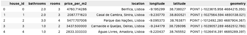
Now that we have a geopandas.GeoDataFrame, we can start adding more information relevant to the house locations. It's time to enrich our data!

Adding Data

Geospatial data usually comes in two types:

• A vector data represented by a shape. This can be a point, a line or a polygon. For example, we create point data from the locations of the houses, and Portuguese parishes can be represented by polygons.
• Another type of data is raster data, and this one is represented as matrices. I will come back to this one later.

Parish Name

House prices can vary a lot depending on location - so we will be adding the name of the parish to each house data.

Vector data file formats can be of .shp (shapefile) or .geojson (geojson) types. Both types can be read using the geopandas API. We will get the parishes data as a shapefile from the Portuguese government website:

Once we have the parish data we can use geoprocessing operations to join with our existing data.

For parishes, we can do a Spatial Join with a 'within' predicate. This means that it will join columns if the house is within the parish.

Hospitals within 1 kilometer radius

Let's do another experiment: counting the hospitals that are within a 1000 meter radius from the houses. We will have to do three different transformations:

1. Creating a buffer of 1000 meters around each house;
2. Doing a spatial join with Hospital data;
3. Grouping the data and counting the number of Hospitals.

To see how this was done, see below:

Distance to closest metro

I have aggregated the metro locations of Lisbon in a CSV file. You can find it here.

I will use their locations to obtain the Euclidean distance to the closest metro station - the method used here was to obtain the closest metro and calculate the distance from the house to that closest metro. Since we are working with locations in meters, the distance result is also in meters:

Elevation

So far, we have been working with vector data and geopandas offers great commands to work with them.

But as I've said, there is also another type of data that is important to learn to work with: raster data. This is a matrix shaped data, used to store continuous surface data, such as the elevation in each point.

In this example, we will be adding the elevation of each house location. Even though it might not be super relevant for this use case, it is still useful to learn how to work with it.

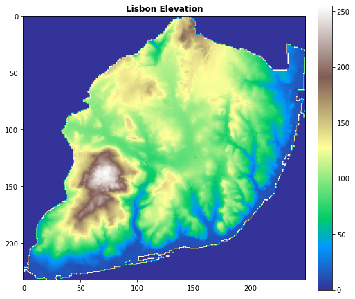
Raster data, like vector data, can have a coordinate reference system associated with it. By using the rasterio library it is possible to read and process this type data. We just have to provide the x and y coordinates to the raster data, and it returns a value which, in this case, will be the elevation:

In the end, we can clear everything we do not need and organize our table with the newly added information.

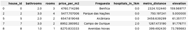
As you can see, by knowing the location of each house, we were able to add a lot relevant information to our dataset. We could also keep exploring open source data for more things to add.

Some Statistics

As a bonus, and now that we have our table ready - let's check some common statistics we can extract from geographical data. First and foremost, doing statistical analysis with geospatial data can entail different techniques which normal statisticians are not used to.

PySal is the Python spatial analysis library, an open source cross-platform library for geospatial data science with an emphasis on geospatial vector data written in Python. It abstracts a lot of the statistical analysis that can be done by aggregating different modules with different approaches.

To cover all that PySAL offers, several other tutorials would have to be written. I will use this one to give a brief introduction on one of the modules: splot. This is the module responsible for performing spatial autocorrelation analysis.

As with any correlation analysis, we need two continuous variables. For our example, our first and main one is the price per m2 of the houses.

The second variable needed is the weights matrix. This is based on contiguity or distance between shapes. PySal has everything required to generate this from a GeoDataFrame in its standard module.

We are working with multiple Point geometries (the house locations), so we can use a distance-based matrix generated using the K-Nearest-Neighbours method.

For this specific problem, we set a high enough K because of overlapping house locations, else, it won’t be able to generate the matrix. The weights for each data point are normalized by setting the transform attribute to “r”.

Once we have calculated the Local Moran autocorrelation, we can give it to a LISA cluster and visualize the Hot Spots.

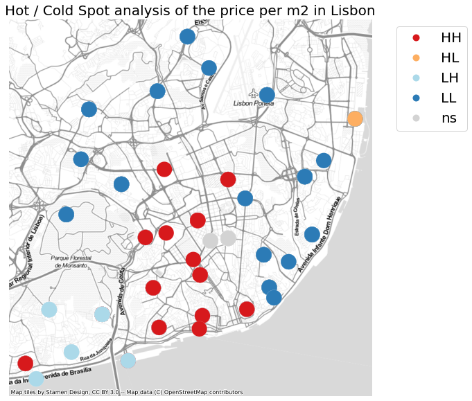
In the visualization above we can observe in red, the Hot Spots (HH), in blue, the Cold Spots (LL), in orange, the Hot Spots surrounded by Cold Spots (HL) and in light blue, the Cold Spots surrounded by Hot Spots (LH). There are also some spots that didn't pass the significance test (ns).

With this simple analysis we can clearly see where the outliers are, and in the case we would like to buy a house in a location where prices are low but are surrounded by others with high prices - this means getting one in the LH spots.

Of course, this would only be a way to highlight some spots, further analysis could still be done, especially with all the extra data we can still add with our geoprocessing toolkit.

Conclusion

By following allong with this tutorial, you have acquired new skills to help you locate your data and boost it with geo-processing! You learnt how to work with GeoPy to help you locate your data, GeoPandas to perform vector data transformations, rasterio to perform raster data transformations, and splot to perform correlation analysis. But there are many more functionalities within these  libraries and other great libraries to explore.

Thank you for reading this post! Feel free to connect with me through LinkedIn and in case you are interested in joining a fantastic team with whom you can learn other cool things such as this, check out DareData Engineering.